| Get your Combat-Fishing Stuff Here! |
| Get your Combat-Fishing Stuff Here! |
Use of a Neural Network with Supervised Learning to Simulate the Feeding Response Behaviour of a Largemouth Bass .
by Bryce L. Meyer
15 April 1996
Table of Contents:
Abstract and Overview
Table of Contents
Introduction
Biological Basis for Simulation
Figure #1a: Largemouth Bass
Sensory Locations
Figure #1b: Bass Receiving
Sensory Data from a Potential Prey
Classification Neural
Networks
Figure #2: A Simplistic
1 Node Neuron
Basic Algorithm
Figure #3a: Input Data Format
Figure #3b: Input Data Form
Experimental Method
Table #1: Test (Training) Items for FILB.
Figure #4: Architecture Used for this Simulation
(FILB)
Table #2: Certification Results for 10 iterations
by case
Conclusion / Suggestions for Future Work
Acknowledgments
References / Bibliography
Attachment #1: Inputs to FILB
Attachment #2: FILB Output File with Weights
Click each item below for source code (will require minor modification
to run)and data files:
QBASIC
Main FILB Code
QBASIC
Binary Converter
QBASIC
Input FIle Maker
QBASIC
Input File Checker
Input Data Files
Ouput
Data FIles
Neural networks are often used as classification algorithms,
and also in the simulation of biological/psychological behavior. In this
case, a three layered network was used to simulate how a largemouth bass
(a black bass of the N. American Sunfish family) reacts to food/non food
items. Twelve items (referred to here as objects) were represented by division
of the object characteristics into visual, aromatic, and auditory areas.
Visual characteristics included fill color breakdown, fill pattern sample,
eye presence, rounded edges, speed in relation to the bass maximum speed,
and motion pseudo-path. Aromatic characteristics included scent component
breakdown (lipid, protein, mineral levels) and over a scent strength. Auditory
breakdown included a sample pseudo-spectrum and volume. A total of 69 binary
bits were required for representation. The output of the network was a
+1 (bite) or -1(avoid) response corresponding to food or non-food object
classification. Incorrect responses forced a back-propagation algorithm
to correct the weights for each layer. The number of neurons for each layer
was 6 and 1, with a sgn(.) activation function for each layer. Ten
iterations with out noise, then 10 iteration with noise, of 11 objects
was used for initial supervised training. Noise injected was to the input
state vector in the form of represented temperature and light levels. Then
an unsupervised test of a ten iterations per object with noise was conducted
for validation with 90% success required for acceptance. Results were that
the network achieved its objective with a 99% success rate.
Back to top
Biological Basis: How does a largemouth bass feed?
Due to the immense popularity of sport fishing for members of the black
bass genus, and particularly for the largemouth bass in the United States,
large bodies of both scientific and pseudo-scientific work have been devoted
to how this aquatic predator feeds. In fact a great deal of personal observation
is used here. Largemouth bass prefer warm fresh to brackish water ponds,
swamps, lakes, and rivers, with large amounts of vegetation, rocks, and
other structure. Due to their aggressiveness and large appetite , they
have mouths that are often 20% of their length, an d will attempt to eat
anything that basically resembles food and is smaller than they are. They
often suspend 2-10 feet below the waters surface or around underwater
structure waiting in ambush for an unwary minnow, frog, insect, salamander,
or even bird to venture within striking distance. When a potential food
object approaches, the bass determines in a second or less, with a combination
of instinct and experience, whether to explosively engulf this object as
prey or to simply watch it pass by. This bite/avoid response is referred
to here as the feeding response or feeding impulse. This response is stimulated
by cues received visually from the eyes , which are very color and pattern
sensitive, aromatically from the nose, which tastes the water for chemical
variations, and auditory from the lateral line, which senses minute vibrations
from an object including the panicked breathing of a smaller fish nearby
(See figure #1).
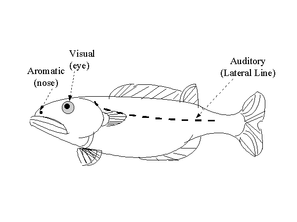
FIGURE #1a: Largemouth Bass Sensory Locations
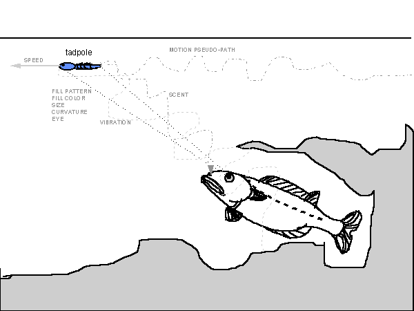
FIGURE 1b. Bass Receiving Sensory Data from a Potential Prey
While determination of these characteristics would seem
simply to be conditional, a basss life is further complicated by many
factors including temperature variations, which alter how readily a bass
will bite (about 75oF seems to be prime for feeding) , and by
light level variations, which determine how well the bass can see. From
observations made by the release of hatchery raised bass into natural conditions,
it has been observed that the bass will initially determine anything smaller
than itself to be food. After a several painful experiences either from
attempting to eat an inedible natural object such a twig or pebble, or
from striking a lure and subsequently being released, the bass will become
more wary and will be able to determine with some certainty which objects
it should or should not eat (unless the bass itself is eaten!).
Back to top
Classification Neural Networks
The feeding response of a bass has only two possible outcomes:
bite or avoid. These outcomes can be regarded as classes, allowing the
use of the classification type of neural networks for simulation. As might
be inferred, classification neural networks, including those using either
perceptrons and/or neurons, determine which of two possible, separable,
classes an input vector x belongs to. Each x component is
multiplied by an associated component of a weighting matrix W, which
is then summed for each neuron, see figure #2 below.
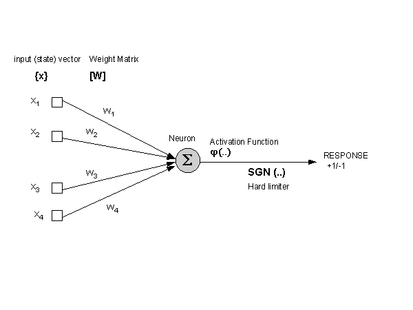
FIGURE #2: A Simplistic One Node Neuron (Similar to figure 1.4 pg. 8 of Ref.#2)
This is usually expressed in matrix form as y=WTx
for each fully connected neuron layer, where W is restricted by S
|W|
=1 for each layer. The response for each neuron is then determined
by the function j(y)+q
where j is the activation function and
q is the threshold constant. For a multi-layered network, the
x for the next layer would the be x=SGN((j(y)+q)+Z)=response
+lags . For each succeeding layer y is found,
then the response is found, the x is set equal to the response plus
lags Z. For the last layer the response is then either one of the classes.
This trip from input x to final response will be termed here as the forward
pass. Lets then assume that the response is not correct. Assuming supervised
learning, where the correct response in known, a feedback can then be used
to indicate this correct response and alter the weights in each layer to
produce the correct response. The changes to W to correspond with this
knowledge can then be found by DW=
b * dj( d - y
)*x + l, where b
is the learning rate parameter and l is a learning
rate offset. This will be called the backwards pass. W for the next
forward pass equals W+DW and the process
is iterated until W remains unchanged (stable) between epochs (one
forward + one backward pass). Using multiple training cases and multiple
epochs, where the network passes through a iteration for each trip through
the training cases, then a suitable neural network may emerge. Suitability
can be determined by certification testing, where the x may be a new case
or a training case with noise, and then the net is iterated to determine
the percentage of correct responses. If this percentage meets the users
minimum criteria then the network is accepted for use. If not accepted
the net may be modified by adding nodes and modifying network constants(b,l,q,
etc.) , then retraining until accepted.
Back to top
BASIC ALGORITHM
Referring back to the explanation of largemouth feeding behavior and to the proceeding discussion of classifying neural networks, an algorithm describing the feeding response in terms of these networks can be developed to simulate this behavior, and a program written to test it. Assuming two layer network , input values to input layer to output layer which gives response, and assuming that the input vector can be represented using total of 69 binary values, and assuming a set of 12 different training cases then the following algorithm is constructed:
Definitions: inp=input values, i = input layer, o=output layer, Respi,case =current response for a current case, Respcorr=correct response for the current case, nnodes= # of nodes in input neuron layer, Z=0
Step 0: read in data representations for each case (69 xinp values, one value for correct response)
Step 1: initialize Wi (a 69x nnode array), Wo (a nnode by 1 array)
Iterate 5 times for all cases (case 1-12 then case 1-12 again, etc.)
* forward pass *
yi = [Wi]T*[xinp]
xi = SGN (j (yi))
yo= [Wo]T*[xi]
Respi,case = SGN (j (yi))+q
if Respi,case = Respcorr,case then goto next case else:
*backward pass *
Dwi =[ [b * dj( Respcorr - yi )]*[xinp]T + l]T
Dwo =[ [b * dj( Respcorr - yo)]*[xi]T + l]T
Wi=Wi+Dwi
Wo=Wo+Dwo
normalize Ws so that S |Wi|=1 and S |Wo| =1.
Repeat forward pass
Step 2: repeat Step 1 iterations for each case for noise caused by Temperature (add .01*| 75-TempoF| to q) and Light Level (scale 0-10, if 10=noon then subtract INT |10-Light Lvl|1/2 from fill color before binary conversion, see next section.)
Step 3: Test using new data or training cases above with noise as in step 2. for at least 10 forward passes ONLY, compare number of correct responses versus incorrect responses.
Step 4: if Step 1,2,3 is unacceptable alter b, or alter l, or then lastly add a node to nnodes (input neuron layer).
COMPLETED, SAVE WEIGHTS AND NET STRUCTURE
The simulation for this paper was constructed using this
algorithm. In order to represent the input data the example form in figure
#3a below was filled out with the data having the following sizes and characteristics
(figure #3b):
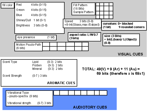
FIGURE 3a: Input Data Format
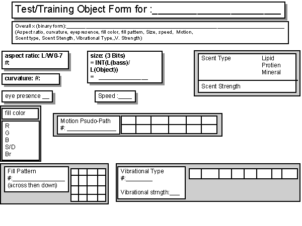
FIGURE 3b: Input Data Form
Once a form is filled for all the data, a package was written in QBASIC Ó to convert the decimal numbers and patterns to a 69 bit binary string, with the correct response indicated (+1=bite, -1=avoid).
Example:
tadpole
100110011111001011011111111111111111111010001010101011010011001100011
+1
This binary string is then converted to +1 for 1 and -1
for zero in the main program as xinp .
Back to top
The goal in the simulation of feeding impulse was to create
a Neural Net program that would accept the input data as above, using the
aforementioned algorithm, that would be above to predict with 90% accuracy,
after training, whether a test item was a food or non-food item (to bite,
or not to bite). The FILB ( Feeding Impulse of a Largemouth Bass) program,
written in QbasicÓ implemented the classification
algorithm. Initially, there were an input layer of 13, two hidden layers
of 6 and 3 neurons, and an output layer of 1 neuron. This architecture
proved very slow and un-trainable on the first iteration of the twelve
test cases listed below.
TABLE 1: TEST ITEMS FOR FILB
|
|
|
|
|
|
|
|
|
|
|
|
|
|
|
|
|
|
|
|
|
|
|
|
|
|
|
|
|
|
|
|
|
|
|
|
Next, the number of layers was reduced to an input layer of 13 nodes, a hidden layer of 6 nodes, and an output node. After numerous alterations of b and l for each layer, as well as switching theta between tanh and simply SGN, this arrangement also proved very difficult to train after two training iterations. Finally, the configuration was reduced to a single input and output layer as shown in figure #4 below.
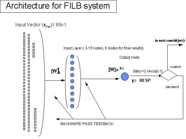
FIGURE #4 : Architecture Used for this Simulation (Feeding Impulse Largemouth Bass)
This configuration proved to be trainable for 10 no-noise
iterations, with bi=.01,
bo=.01,
j
= sgn (y) . This configuration in some ways represents a multiple
layer perceptron arrangement. After surviving initial non-noise training,
random noise for light level and temperature was added to the visual characteristics
(first 49 bits) , and temperature noise was inflicted on the scent characteristics
(next 11 bits) . This training was conducted successfully, so the code
with the trained weights was tested for certification for the forward pass
only for 10 iterations per object with random noise as above . The table
below has the certification results for each case. From Attachment #2,
the hidden layer weights [W]o are all the same, inferring
that this layer may have been unnecessary here, but in more complex cases
they might have been necessary.
TABLE #2: CERTIFICATION RESULTS FOR 10 iterations by case
|
|
|
|
|
|
|
|
|
|
|
|
|
|
|
|
|
|
|
|
|
|
|
|
|
|
|
|
|
|
|
|
|
|
|
|
|
|
|
The final weights are shown in Attachement #2. The actual input data in shown in Attachment #1.
As a result of the >90% certification results, the model
is a satisfactory simulator of the feeding behavior of the largemouth bass
given the simplicity of the model. Note that resulting matrix in the
attachments show that a single layer net would produce identical results.
Future
applications of this model could include expanding the input data for each
case and adding a better input program that might be linked to a digital
video camera, underwater microphone, and aromatic sensors such as a pH
gauge and Electrolyte meter. These sensors, implemented with an improved
neural network model could be used by major lure manufacturers to test
new lures before production, and by professional fishermen to improve their
fishing techniques during northern winters. Since the simple model performed
very swiftly ( 110 cases with noise generation in under 1 minute) when
using QBASICÓ and ran on a 80386DX laptop
system, a system with an 80586 or similar processor system using an efficient
compiler with multimedia input capabilities would be sufficient for the
more complex model, provided the input did not exceed around 250 inputs
(speed slows greatly with improved size of W). Though this future system
would seem relatively complex, it could still never truly match the performance
of the natural animal, and never quite remove the thrill experienced by
those who pursue it.
Decomposition of the input data and representation of
the vibrational spectra was borrowed with some adaptation from a paper
by J.A. Anderson entitled "Radar Signal Categorization Using a Neural Network".
While most of the bass behavior represented here was obtained by personal
observations during many Saturdays on the water, some information was added
by years of reading magazines such as Missouri Conservationist, Field&Stream,
Fishing, Facts, Sports Afeild, and books by Zane Grey and Isaac Walton.
1. "Radar Signal Categorization Using Neural Networks"
by J.A. Anderson et al., Proceedings of the IEEE, vol. 78 no. 10, October
1990, IEEE Press, Inc. 1990
2. Neural Networks: A Comprehensive Foundation, S. Hayken,
Macmillian College Publishing,Inc., NY, 1994
Format:
Object NAME
Binary Input string (69 bits long)
Food/Not food correct response (+1=food,-1=not food)
tadpole
100110011111001011011111111111111111111010001010101011010011001100011
1
shiner
100110100100101110101111110100000000001111011111110100101110101010100
1
crankbait
101110100101111110110111110101010000001110111001100000100110101010110
-1
lillypad
001100010111100101011111111111111111100111100000000001101000000000000
-1
twig
111000101010101011011111111111111111101011100000000001101100000000000
-1
earthworm
111101010100010001100101010101010101001011011100001011011000011100001
1
bluegill
010111010101001001100111101010101010101110011001110100110011001100100
1
spoon
011101111111111110110111111111111111111010110101000001000111001100010
-1
log
110000110011000111001111111111111111100011100000000000101000000000000
-1
pebble
001100101010101011001101001011010010111111100000000001001000000000000
-1
chub
101110011101110111011111111111010000010001010101011100110011001100100
1
FILB Success file
Betai= .01
Betao= .01
Test Results
tadpole 90
shiner 100
crankbait 100
lillypad 100
twig 100
earthworm 100
bluegill 100
spoon 100
log 100
pebble 100
chub 100
TOTAL-------- 99.09089 %
Hidden layer Weights
.1666667
.1666667
.1666667
.1666667
.1666667
.1666667
ATTCHMENT #2 (Continued) Input layer Weights
.011359 .011359 .011359 .011359 .011359 .011359
6.03805E-03 6.03805E-03 6.03805E-03 6.03805E-03 6.03805E-03 6.03805E-03
-.0323786 -.0323786 -.0323786 -.0323786 -.0323786 -.0323786
4.487573E-03 4.487573E-03 4.487573E-03 4.487573E-03 4.487573E-03 4.487573E-03
1.503475E-02 1.503475E-02 1.503475E-02 1.503475E-02 1.503475E-02 1.503475E-02
1.480656E-02 1.480656E-02 1.480656E-02 1.480656E-02 1.480656E-02 1.480656E-02
-2.789193E-02 -2.789193E-02 -2.789193E-02 -2.789193E-02 -2.789193E-02 -2.789193E-02
.0222181 .0222181 .0222181 .0222181 .0222181 .0222181
4.847874E-04 4.847874E-04 4.847874E-04 4.847874E-04 4.847874E-04 4.847874E-04
2.382966E-02 2.382966E-02 2.382966E-02 2.382966E-02 2.382966E-02 2.382966E-02
-2.073499E-02 -2.073499E-02 -2.073499E-02 -2.073499E-02 -2.073499E-02 -2.073499E-02
-2.998738E-02 -2.998738E-02 -2.998738E-02 -2.998738E-02 -2.998738E-02 -2.998738E-02
-6.672164E-03 -6.672164E-03 -6.672164E-03 -6.672164E-03 -6.672164E-03 -6.672164E-03
-.0198549 -.0198549 -.0198549 -.0198549 -.0198549 -.0198549
2.583479E-03 2.583479E-03 2.583479E-03 2.583479E-03 2.583479E-03 2.583479E-03
-4.893496E-03 -4.893496E-03 -4.893496E-03 -4.893496E-03 -4.893496E-03 -4.893496E-03
-1.171188E-02 -1.171188E-02 -1.171188E-02 -1.171188E-02 -1.171188E-02 -1.171188E-02
9.694397E-03 9.694397E-03 9.694397E-03 9.694397E-03 9.694397E-03 9.694397E-03
1.137839E-02 1.137839E-02 1.137839E-02 1.137839E-02 1.137839E-02 1.137839E-02
-.0323786 -.0323786 -.0323786 -.0323786 -.0323786 -.0323786
1.238538E-02 1.238538E-02 1.238538E-02 1.238538E-02 1.238538E-02 1.238538E-02
8.242772E-03 8.242772E-03 8.242772E-03 8.242772E-03 8.242772E-03 8.242772E-03
6.266237E-03 6.266237E-03 6.266237E-03 6.266237E-03 6.266237E-03 6.266237E-03
-7.341745E-03 -7.341745E-03 -7.341745E-03 -7.341745E-03 -7.341745E-03 -7.341745E-03
2.537447E-03 2.537447E-03 2.537447E-03 2.537447E-03 2.537447E-03 2.537447E-03
.011359 .011359 .011359 .011359 .011359 .011359
9.694397E-03 9.694397E-03 9.694397E-03 9.694397E-03 9.694397E-03 9.694397E-03
.011359 .011359 .011359 .011359 .011359 .011359
-8.52776E-04 -8.52776E-04 -8.52776E-04 -8.52776E-04 -8.52776E-04 -8.52776E-04
-3.544179E-02 -3.544179E-02 -3.544179E-02 -3.544179E-02 -3.544179E-02 -3.544179E-02
-2.756867E-03 -2.756867E-03 -2.756867E-03 -2.756867E-03 -2.756867E-03 -2.756867E-03
-2.489462E-02 -2.489462E-02 -2.489462E-02 -2.489462E-02 -2.489462E-02 -2.489462E-02
-2.756867E-03 -2.756867E-03 -2.756867E-03 -2.756867E-03 -2.756867E-03 -2.756867E-03
-1.018781E-02 -1.018781E-02 -1.018781E-02 -1.018781E-02 -1.018781E-02 -1.018781E-02
-2.756867E-03 -2.756867E-03 -2.756867E-03 -2.756867E-03 -2.756867E-03 -2.756867E-03
2.335891E-03 2.335891E-03 2.335891E-03 2.335891E-03 2.335891E-03 2.335891E-03
-2.756867E-03 -2.756867E-03 -2.756867E-03 -2.756867E-03 -2.756867E-03 -2.756867E-03
4.847874E-04 4.847874E-04 4.847874E-04 4.847874E-04 4.847874E-04 4.847874E-04
4.560013E-03 4.560013E-03 4.560013E-03 4.560013E-03 4.560013E-03 4.560013E-03
-1.14531E-03 -1.14531E-03 -1.14531E-03 -1.14531E-03 -1.14531E-03 -1.14531E-03
-.0167322 -.0167322 -.0167322 -.0167322 -.0167322 -.0167322
3.676481E-02 3.676481E-02 3.676481E-02 3.676481E-02 3.676481E-02 3.676481E-02
-5.359838E-02 -5.359838E-02 -5.359838E-02 -5.359838E-02 -5.359838E-02 -5.359838E-02
2.382966E-02 2.382966E-02 2.382966E-02 2.382966E-02 2.382966E-02 2.382966E-02
2.583479E-03 2.583479E-03 2.583479E-03 2.583479E-03 2.583479E-03 2.583479E-03
4.355679E-02 4.355679E-02 4.355679E-02 4.355679E-02 4.355679E-02 4.355679E-02
3.483431E-02 3.483431E-02 3.483431E-02 3.483431E-02 3.483431E-02 3.483431E-02
1.130596E-02 1.130596E-02 1.130596E-02 1.130596E-02 1.130596E-02 1.130596E-02
2.583479E-03 2.583479E-03 2.583479E-03 2.583479E-03 2.583479E-03 2.583479E-03
2.485604E-02 2.485604E-02 2.485604E-02 2.485604E-02 2.485604E-02 2.485604E-02
1.300849E-02 1.300849E-02 1.300849E-02 1.300849E-02 1.300849E-02 1.300849E-02
3.540321E-02 3.540321E-02 3.540321E-02 3.540321E-02 3.540321E-02 3.540321E-02
.0111044 .0111044 .0111044 .0111044 .0111044 .0111044
5.572265E-04 5.572265E-04 5.572265E-04 5.572265E-04 5.572265E-04 5.572265E-04
-8.009726E-03 -8.009726E-03 -8.009726E-03 -8.009726E-03 -8.009726E-03 -8.009726E-03
2.043944E-02 2.043944E-02 2.043944E-02 2.043944E-02 2.043944E-02 2.043944E-02
2.431355E-02 2.431355E-02 2.431355E-02 2.431355E-02 2.431355E-02 2.431355E-02
-8.576256E-03 -8.576256E-03 -8.576256E-03 -8.576256E-03 -8.576256E-03 -8.576256E-03
1.503475E-02 1.503475E-02 1.503475E-02 1.503475E-02 1.503475E-02 1.503475E-02
1.473411E-02 1.473411E-02 1.473411E-02 1.473411E-02 1.473411E-02 1.473411E-02
-8.576256E-03 -8.576256E-03 -8.576256E-03 -8.576256E-03 -8.576256E-03 -8.576256E-03
7.37561E-03 7.37561E-03 7.37561E-03 7.37561E-03 7.37561E-03 7.37561E-03
2.755846E-02 2.755846E-02 2.755846E-02 2.755846E-02 2.755846E-02 2.755846E-02
3.098661E-02 3.098661E-02 3.098661E-02 3.098661E-02 3.098661E-02 3.098661E-02
-8.576256E-03 -8.576256E-03 -8.576256E-03 -8.576256E-03 -8.576256E-03 -8.576256E-03
-5.148096E-03 -5.148096E-03 -5.148096E-03 -5.148096E-03 -5.148096E-03 -5.148096E-03
1.130596E-02 1.130596E-02 1.130596E-02 1.130596E-02 1.130596E-02 1.130596E-02
-4.110109E-02 -4.110109E-02 -4.110109E-02 -4.110109E-02 -4.110109E-02 -4.110109E-02
.0111044 .0111044 .0111044 .0111044 .0111044 .0111044
| Get your Combat-Fishing Stuff Here! |